Figure S1. Left panel: solar prominence (Big Bear Solar Observatory). Right panel: solar filament (Hida Observatory, Magara & Kitai 1999).
Gas density and temperature in the filament/prominence are typically 100 times higher and lower than those of a surrounding coronal plasma, respectively, so pressure equilibrium between a filament/prominence plasma and coronal plasma may be established. Although it is surrounded by the hotter and less dense coronal plasma, and affected by the solar gravitational field, the filament/prominence tends to have a relatively long, stable phase during which its global shape slowly changes, while small-scale internal motions such as upflows, downflows, and circulating flows are continuously observed in it.
Classical models (two-dimensional, static)
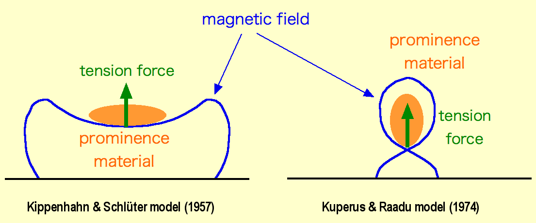
What magnetic field configuration in the filament/prominence can be assumed is important because this may explain its relatively long, stable phase. Since gas pressure scale height in the filament/prominence is usually much smaller than its observed vertical extent, gas pressure gradient force may not support the filament/prominence plasma against the gravity. On the other hand, Lorentz force (= magnetic pressure gradient force + magnetic tension force) that depends on strength and configuration of magnetic field is a possible candidate for supporting that plasma.
The filament/prominence tends to exist above a polarity inversion line (PIL) in a solar surface (photosphere), which separates a positive magnetic polarity region from a negative one. A narrow region along the PIL is called a filament channel. This suggests that the magnetic field may have a bipolar configuration in the filament/prominence, and two types of two-dimensional static models with different bipolar configurations are considered: normal polarity model and inverse polarity model (Figure S2). In both models the magnetic tension force supports the filament/prominence plasma against the gravity.
The two-dimensional magnetic configurations assumed by the classical models may represent different aspects of three-dimensional magnetic structure of the filament/prominence (Figure S3).
Figure S3. Three-dimensional magnetic structure gives different two-dimensional magnetic configurations, depending on viewing positions. From a lecture slide. For more than a cartoon, see this.
Figure S4. Schematic explanation of flux rope on the Sun and its projected view (magnetic island, two-dimensional configuration) on a vertical plane. From a slide presented at AOGS meeting.
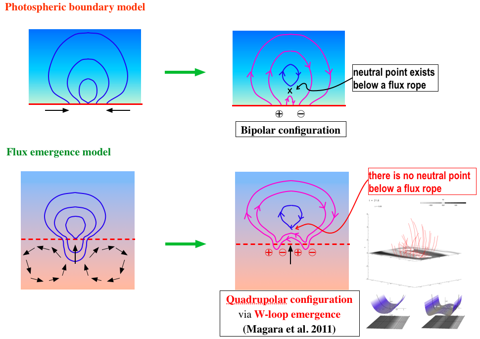
There are two types of models that explain how to form the flux rope: i) Photospheric Boundary model (PB model) and ii) Flux Emergence model (FE model). In the PB model photospheric processes play a key role in forming the flux rope, where subsurface magnetic fields and subsurface plasma motions are not taken into account. In the FE model the emergence of a twisted magnetic flux tube associated with subsurface convective motions plays a key role in the formation of the flux rope (Figure S5).
Figure S5.Photospheric boundary model (PB model; top panel) and Flux emergence model (FE model; bottom panel). From a slide presented at AOGS meeting.
We then explain similarity and difference between the PB and FE models.
In the PB model a photospheric converging flow (top panel of Figure S6) causes magnetic reconnection in the photosphere, which is regarded as one of possible mechanisms for producing flux cancellation. This leads to forming the flux rope, or magnetic island composed of closed field lines on a projection plane (right panel in Figure 4S and top panel of Figure S6).
Figure S7. Magnetic configurations assumed by PB model (top panel) and FE model (bottom panel). From a slide presented at AOGS meeting.
Click here to enlarge. Figure S8: Formation of quadrupolar-like structure via W-loop emergence (Magara et al. 2011). In the left panel inner and outer field lines of emerging twisted flux tube are drawn in blue and red, respectively. The inner field lines compose the flux rope while the outer field lines become Ω-loops overlying the flux rope and W-loops underlying it (see also the bottom-right panel in Figure S7). In the right panel the red arrows represent the transverse component of photospheric magnetic field, while the gray-scale map shows the distribution of vertical magnetic flux density in the photosphere. Note that the PIL rotates as W-loop emergence proceeds.
Fine structure of filament
High-resolution observations revealed fine structure of the filament (Martin 1998; Figure S9), represented by satellite/parasitic polarity regions and barbs (filament feet). This implies that the above-mentioned quadrupolar-like structure may be formed around the filament channel.
Figure S9. Fine structure of filament (Martin 1998).
The barbs often show chirality of the filament (Figure S10). The chirality may be related to handedness of an emerging twisted flux tube that forms magnetic structure of the filament (left-handed field-line twist => dextral filament, right-handed field-line twist => sinistral filament).
Figure S10. Chirality of filament (Pevtsov et al. 2003).
The barbs tend to appear sporadically along the filament channel, which suggests that the twisted flux tube may emerge in an undulated shape, as shown at the top panel (time = 5) of Figure S11 (see also Magara 2007). Inner field lines of the undulated flux tube compose the main body of the filament (spine), while its outer field lines form an overlying coronal arcade above the main body (time = 33 at the top panel) and dip-like structure below the main body (bottom panel of Figure S11). A massive plasma could accumulate in the dip-like structure to produce the barbs.
Evolution of an emerging magnetic field is generally characterized by three distinct phases: emergence, formation, and eruption. The 2nd phase is relatively long and stable, during which the magnetic structure of the filament/prominence may be formed and evolve gradually. From a stability viewpoint, the magnetic configuration assumed by the PB model could be unstable because the neutral point exists below the flux rope, where magnetic reconnection is expected to occur (see left panel of Figure S12). On the other hand, the magnetic configuration assumed by the FE model coud be stable because no neutral point exists below the flux rope, which is suitable for the long-lasting formation phase (see bottom-right panel of Figure S12). What causes a transition from the quasi-static formation phase to the eruption phase is discussed in terms of κH mechanism (Magara 2013; An & Magara 2013).
Figure S12. Stability of flux rope in PB and FE models. From a slide presented at AOGS meeting.